Real Estate Price Prediction via Machine Learning: A Case Study of Pakistan’s Cities

Introduction

The real state has emerged swiftly in Pakistan in the last two decades due to housing societies and it is currently playing a vital role in the economy of Pakistan via large tax collections. Real estate has become a tower of strength in the Pakistani economy. It is improving the way of life by enhancing the infrastructure of the dwelling. Many people work their entire lives to buy a house for their family to transition from renting to owning a home. Global urbanization has expanded significantly in the past two decades, which has led to increased residence demand in metropolitan areas and higher real estate prices.

The purpose of this paper is to make it easy for buyers to buy a new house and to help them negotiate with a society’s real estate agents on the price of a house in metropolitan areas. In addition, the dwelling price forecasting model can lead to investing in the real estate business. In this research paper, supervised learning is used to forecast the price of the house by implementing various Machine learning algorithms.

Machine learning is a subdivision of AI and is sometimes referred to as a statistical technique that focuses on algorithms that are capable of learning from data to make predictions and decisions by extracting meaningful patterns and relationships in the data. Although Machine learning is unable to constantly generate precise predictions, we made every effort to get good results.

There are the following Machine learning algorithms implemented on a secondary dataset that is obtained from the open real estate portal of Pakistan¹: SGDRegressor, Decision Tree, Gradient Boosting Reg ressor, XGB Regressor, AdaBoost Regressor, Random Forest Regressor, CatBoost Regressor, KNN, LightGBM Regressor, and Stacking regression. The dataset holds data from 2018–2019 for the following metropolitan areas: Lahore, Islamabad, Karachi, Rawalpindi, and Faisalabad.

However, the model is built for Lahore, Islamabad, Karachi, and Rawalpindi. The model was trained on static training with two different ratios. We evaluate the ML algorithms on a dataset and show the benchmarks of the algorithms. Segment 2 illustrates the literature review and segment 3 explains the technique that has been used in the paper. Segment 4 in the paper illustrates the discussion and results. Segment 5 illustrates the conclusion of the whole paper.

Literature Review  

In a volatile real estate business, what are the few effective techniques for predicting house prices? This question always lies in the brain of every buyer, seller, investor, and researcher to make good decisions. Machine learning is a fantastic tool to get a fair prediction. L. Rampini investigated the two cities of the Italian market i.e. Brescia and Varese by using ElasticNet, XGBoost, and an Artificial Neural Network to estimate the price of a dwelling.² The ElasticNet performed worse and got a high mean absolute error (MAE). On the other hand, XGBoost gets a low MAE for both cities.

However, ANN got the lowest MAE and diminished the errors by five percent towards XGBoost outcomes. Researchers also suggested that the prices of houses higher than 800,000 euros would drop from the test dataset. The model trained on identical ANN. Therefore, MAE is reduced by 10% for both cities’ datasets.

The house price can be affected by various factors like how many bedrooms, baths, the house size, etcetera. Maida proposed a model using GXBoost with an excellent accuracy of 98 percent and with an MAE of 22502.08.³

Quang Truong implemented various Machine learning techniques for forecasting dwelling prices.⁴ With some tools, housing economists estimated changes in the rate of interest repayment, and housing affordability in particular geo-locations. Quang Truong predicted the “Housing price in Beijing” and the dataset has rows of 231962 after cleaning data with 19 features.

In data analysis, the author discovered an amazing pattern: the oldest cities are concentrated densely in the center of Beijing, while the newest ones are spread in the sub-urban areas in small numbers. The most expensive house is close to the center of Beijing. The data split ratio in model selection is 4:1 with the scikit learn package. The evaluation function in this project was root mean square logarithmic error. The author used three algorithms, random forest, XGBoost, Light Gradient boosting machine, hybrid regression, and stacked Generalization (it is an ensemble technique).

The results suggested that the stacked generalization regression has a low error on the test set with the value of 0.16350; the random forest has good accuracy in the training set, but it fails to capture the complexity on the test set. Hybrid regression also has good accuracy on the test set with a value of 0.16372.

Y. Feng compared the approaches of multilevel modeling and artificial neural network accuracy approaches to standard hedonic prices to capture location and their explanation.⁵ The baseline was a hedonic price model that compared with MLM and ANN. The variance summarizes that detached houses are much more expensive as compared to non-detached houses.

Neural networks mapping on each other helps to capture non-linearity from the dataset. The ANN application did not always have good accuracy, but some researchers believed that it had good accuracy. The study was conducted in the Greater Bristol area, which had a wide range of urban and rural mixtures. The data split for training is from 2001–2012, and the test dataset is from 2013. The author concluded that multilevel modeling models have good accuracy.

In this model, Cekic explored different models Linear Regression analysis, random forest regression analysis, Decision tree regression, XGB regressor, and Extra tree regressor.⁶ For model evaluation, there are three metrics used. MAE, RMSE, and R² error. The author trained the model using a training dataset. For accuracy purposes, Extra trees regressor the best accuracy on the test set. But other algorithms also showed good results or performance on the model. After applying PCA (principal component analysis) to a dataset, the features are reduced due to PCA. PCA was applied to select highly discriminative features. Now model again, train, and test on the testing set. The metric score of algorithms is 90 plus percent.

Park and Bae began a trip to real estate by utilizing the power of machine learning to reveal the estimated property pricing.⁷ Their research focused on the growing property market in Fairfax County, Virginia, where 5359 townhouses revealed their secrets to the Metropolitan Regional Information Systems and Multiple Listing Service. To predict the mysterious future of housing prices, the researchers take off their data scientists’ hats and utilize the following algorithms: C4.5, RIPPER, Nave Bayesian, and AdaBoost. The authors checked these algorithms on the test dataset to determine which algorithm prediction was the most precise. As the dust settled, the winning RIPPER algorithm demonstrated its mettle, standing tall as the unrivaled champion of house price prediction.

M Chen investigated ZhaoQing City for house price forecasting grounded on Pearson correlation and multiple regression analysis on several variables.⁸ This paper used ML and statistical theory to research house costs in Zhaoqing City from 2010-2020. The goal was to accurately predict house prices in Zhaoqing City in 2021 and beyond, achieving better similar and precise predictive results. 

House prices in China have significantly increased in the past two decades. In this model, the author hypothesized, that all X-attributes of data can affect the price of a city. However, Chen implemented a T-test, F-test, and ANOVA test for correlation. R² was used to analyze the size of the model fit and chose the finest prediction model for predicting future property values in Zhaoqing City. The model has achieved an accuracy of 0.999. 

Iwona Forys compares the two models (Regression V/s ANN) by applying them to a dataset of Western Poznan.⁹ The ANN exhibits more prominent results as compared to the Regression. Xu employed ANN on second-hand house price data for the forecasting in the ten cities of China and their final models performed consistently, even in complicated market environments, with an average relative root-mean-square error of 0.8%.¹⁰

The nonlinear autoregressive model was implemented using a two-layer feed-forward neural network with a sigmoid activation function in the hidden layer and a linear activation function in the output layer. It was designed for time-series data. During training, the output values were used in an open-loop manner, making the resulting architecture pure feed-forward and potentially more accurate and efficient.

F. Wang deployed the ARIMA model (time series forecasting model) for dwelling price estimation.¹¹ They used a neural network with the activation function ReLu and ADAM optimizer. The author created four hidden layers of neural networks.  The model got a low MRE as well as RMSE as compared to the SVR model. Peddi exploited linear regression on the California dataset for predicting house prices, applying regularization to avoid overfitting and removing outliers from the dataset to avoid bias.¹²  The model accuracy measured by R² was 0.91.

Abigail¹³ and Joshi¹⁴ both used the Random Forest ML technique on the Boston housing dataset. The author employs a data normalization technique. So, the attributes are on the same scale. Both get low MSE and RMSE, which means Random Forest performs very well in predicting the house price.

Xiaojie suggested time series models by operating these three ML algorithms: Levenberg-Marquardt, Bayesian Regularization, and Scaled Conjugate Gradient.¹⁵ The algorithms were applied to a dataset that holds records for 99 cities in China from 2010-2019. The models show a stable performance of 1% average relative root mean square error across all cities in the training, validation, and testing phases with the guidance of Levenberg-Marquardt, which contains four delay neurons and three hidden units.

Wang probed to forecast the direction of the resale price index, applying the Levenberg-Marquardt algorithm for prediction.¹⁶ The accuracy was achieved on distinct architecture on the dataset and finally obtained accuracy from 0.90979 by evaluating through R² error. In addition, Dynamic ANN performs well compared to Static ANN. Jiang focused on Back Propagation i.e. ANN by using the Keras deep learning framework.¹⁷

The DL technique was executed on second-hand Houses in Shanghai, China. Researchers used three hidden layers with an elu activation function; they utilized the optimizer RMSprop with a learning rate of 0.001 and the model achieved the highest accuracy of 0.9559.

Methodology

Data Cleaning

For foresting purposes, we use Python 3.9 and Python libraries. The secondary dataset consists of the following columns property_id, location_id, page_url, property_type, price, location, city, province_name, latitude, longitude, bath’, area, purpose, bedrooms, date_added, agency, agent, Area Type, Area Size, Area Category, the figure 1 is showing after removing outliers and useless columns from the dataset.

We removed location_id, page_url, agency, agent, Purpose, date_added, location (housing societies, and streets name), and Purpose from the dataset. After cleaning the data, we obtained the following data. To ensure maximum accuracy, we use many machine learning algorithms to get a better-predicted value

Data Analysis

EDA is an important step before creating a continuous value prediction model. It helps to discover the pattern from the dataset that may guide towards the best algorithm. If the number of bedrooms and washrooms increases, then the price will increase too as shown below.

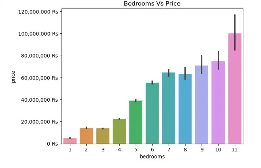
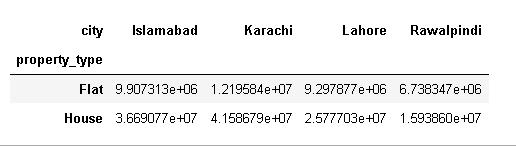
The size category of the house also increases the price. In this paper, we explore the real estate market of four big cities of Pakistan i.e. Islamabad, Lahore, Karachi, and Rawalpindi, and compare the mean price of the houses and flats corresponding to the city.

Data Normalization

Data normalization is a key preprocessing step in Machine learning since it guarantees that every attribute is on the same scale and minimizes the possible effects of changes in the magnitude of all columns. Data normalization ensures that machine learning algorithms are not biased towards features and enhances ML algorithms’ stability and convergence. In this research paper, we use the Min-Max Scaling method by using the scikit-learn library, and the mathematical formula is given below

                                     X _Normalized = (𝑋 – 𝑋𝑚𝑖𝑛)/(𝑋𝑚𝑎𝑥 – 𝑋𝑚𝑖𝑛)

Where X = data of each attribute 

X_min = Minimum value of each attribute X_max= Maximum value of each attribute.

Partition of a Dataset

The dataset is divided into two sections which are training and testing, using the scikit-learn function train_test_split. The training dataset is used to train the model, and the test set is used to forecast the trained model’s accuracy. The data is divided into two ratios.

• 75% for the training and 25% for the testing
• 85% for the training and 15% for the testing

Metric for evaluation

There are many routes to check the accuracy of the model but in this research paper, we use two metrics for model evaluation. 

R² Score

A useful metric for evaluating the goodness of it for a regression model. The amount of variance explained by the independent variables in the dependent variable (goal) can be determined, as to how well this model fits the observed data points. In this paper, we evaluate R² by using the scikit learn library. 

Mean Absolute Percentage Error (MAPE)

The mean percentage difference between forecast and actual values is calculated. In this paper, we evaluate the MAPE by using the scikit learn library.

Machine Learning Algorithms

In this research, we applied numerous supervised Machine learning algorithms for better performance. The target attribute has a continuous value; therefore, we used regression algorithms. All algorithms are hyperparameters tuned by a GridSearchCV feature of Scikit-learn.

Stochastic Gradient Descent (SGD)

The SGD optimizes the model’s coefficients by iteratively adjusting them to minimize the mean square error and make it suitable for linear regression problems. The hyperparameters used in this specific instance of the algorithm include the regularization strength (alpha=0.04), the initial learning rate (eta0=0.08), the learning rate schedule (‘invscaling’), the maximum number of iterations (max_iter=213), and the type of regularization penalty (‘l1’).

Decision Tree

It is a regression algorithm that constructs a decision tree to model relationships in data. With “auto” as the criterion for selecting the maximum number of features, it determines the best splitting strategy based on data characteristics. It sets a minimum of 7 samples per leaf and requires a minimum of 5 samples to split an internal node, ensuring a balance between model complexity and generalization. The maximum depth of the tree is limited to 12 levels, controlling its overall size. This configuration allows the Decision Tree Regressor to effectively capture complex patterns in data while preventing overfitting.

Gradient Boosting Regressor

It belongs to the boosting family of assemble methods of ML. It leverages a learning rate of 0.099 to control the contribution of each tree in the ensemble mechanism. With a maximum depth of 9, it allows for intricate feature interactions. Considering the square root of features (‘sqrt’) ensures diversity among base estimators. A minimum of 3 samples per leaf and a minimum of 4 samples to split internal nodes to strike a balance between model complexity. With 280 estimators can effectively capture complex patterns.  The ‘warm_start’ parameter is set to false,’ indicating that the training process starts from scratch rather than building upon previous iterations.

XGBRegressor

It uses the Gradient Boosting architecture to develop ML algorithms and provides parallel tree boosting. A gamma value of 0 implies no regularization of the split decisions, while a learning rate of 0.089 controls the step size during optimization. With a maximum depth of 16, that allows for the capture of complications from the dataset. A minimum child weight of 25 ensures that each leaf node has a minimum number of instances, contributing to model stability. A regularization term with lambda=12 is also applied, further controlling model complexity.

AdaBoost Regressor

Adaboost regressor belongs to the boosting family of assemble methods of ML that combine multiple weak learners to design a strong learner. It employs a low learning rate of 0.01, which controls the step size during optimization to ensure gradual learning. With 214 estimators, it combines the predictions of multiple base estimators (the Decision Tree Regressor in this case) to make more accurate predictions. Each base estimator is constrained to a maximum depth of 14 to prevent overfitting. Additionally, it utilizes the ‘exponential’ loss function, with the weights being updated after every boosting epoch. This combination of hyperparameters makes the AdaBoost Regressor a powerful tool for predicting the price of real estate in the Pakistani market.

Random Forest Regressor

It creates multiple decision trees during training, combines the mean of every decision tree result, and finally predicts a continuous value. Therefore, it is known as the bagging method, a branch of the ensemble method. We set bootstrap true and each tree is constructed with random subsets of features, reducing overfitting. The algorithm consists of 205 estimators, each considering a minimum of 6 samples for splitting nodes and a minimum leaf size of 1. The ‘sqrt’ option for max_features ensures controlled randomness in feature selection, while the OOB (Out-of-Bag) score provides an internal validation metric.

CatBoost Regression

CatBoost is a gradient boosting library for ML, and this model consists of hyperparameters: a tree depth of 9, 180 iterations, a regularization parameter of 0.28708134 for L2 regularization, a learning rate of 0.0999, and a model size regularization parameter of 0.1.

KNeighbors Regressor

It simply memorizes the training data. When we want to estimate an unknown data point, the algorithm identifies the k-nearest data points from the trained dataset for the unknown point, computes the average of the k-nearest points (k=6) from the train data, and returns the predicted target value.

LightGBM Regressor

LightGBM is a gradient-boosting framework that utilizes tree-based learning approaches. It has swift training and high efficiency. LightGBM employs histogram-based algorithms to bucket continuous feature values. It produces an ensemble of decision trees with a learning rate of 0.2 and a maximum depth of 12, efficiently capturing complicated relationships in the data. To avoid overfitting, it utilizes a minimum of 9 samples per leaf node (min_child_samples) and builds 300 trees (n_estimators) with 14 leaves each (num_leaves). It also employs regularization with a lambda of 0.50314465 (reg_lambda) to control model complexity and avoid overfitting.

Stacked Generalization

Stacking is a type of ensemble method but it combines strong and heterogeneous learners. It combines three diverse base models: a RandomForestRegressor, a GradientBoostingRegressor, and a KNeighborsRegressor, each with its set of hyperparameters that have been trained for the previous model and the final ensemble, constructed using a LinearRegression meta-model, aggregates the predictions from the base models. 

Results and Discussion

We ran Machine learning algorithms and achieved benchmarks in training and testing. However, higher accuracy is attained on the train set, but we consider the benchmarks that have been derived on a test set. The ensemble technique performs marvelously as compared to the other learners. Regressor and CatBoost Regressor perform well in the case of R² on either test set, but they don’t perform well in the case of mean absolute percentage error (MAPE) as compared to other ensemble methods.

XGB, Gradient Boosting Regressor, and AdaBoost Regressor perform well on the trained and test sets in both evaluations, that is, R² and MAPE. The random forest ML algorithm obtained extraordinary benchmarks in R² and mean absolute percentage error as compared to all previous algorithms. Stacking performs marvelously in all aspects, like the different ratios of trained and tested sets and on either evaluation method. However, random forest evaluation accuracy is close to stacking, but ultimately, the winner is stacking.

0.15 TEST SET		Accuracy on Test Set		Accuracy on Train set
Algorithms		Mean Absolute Percentage Error	R2 Error	Mean Absolute Percentage Error		R2 Error
SGD Regressor		0.7088	0.7099	0.7007		0.7119
Decision Tree		0.2551	0.8719	0.2403		0.8965
Gradient Boosting Regressor		0.2042	0.917	0.1735		0.9683
XGB Regressor		0.199	0.9033	0.1764		0.9104
AdaBoost Regressor		0.2109	0.9103	0.1797		0.9709
Random Forest Regressor		0.1878	0.9106	0.1115		0.9555
CatBoost Regressor		0.2541	0.9059	0.2486		0.9311
Light GBM Regressor		0.2437	0.911	0.2394		0.9346
Stacking Regressor		0.1877	0.9157	0.1355		0.9696
KNN Regressor		0.3205	0.7996	0.2665		0.8415

0.25 test set		Accuracy on Test Set		Accuracy on Train set
Algorithms		Mean Absolute Percentage Error	R2 Error	Mean Absolute Percentage Error		R2 Error
SGD Regressor		0.6891	0.7245	0.6839		0.7026
Decision Tree		0.2529	0.8707	0.2348		0.8917
Gradient Boosting Regressor		0.2029	0.9108	0.1691		0.9701
XGB Regressor		0.1972	0.9019	0.1703		0.9094
Ada Boost Regressor		0.209	0.9075	0.1752		0.9722
Random Forest Regressor		0.1868	0.9076	0.1106		0.9517
Cat Boost Regressor		0.2558	0.9053	0.2469		0.9323
Light GBM Regressor		0.2428	0.914	0.2348		0.9341
Stacking Regressor		0.1868	0.9153	0.1388		0.9696
KNN Regressor		0.322	0.8033	0.2653		0.8327

Conclusion

People are concerned about the cost estimation of a house or flat. Cost estimation is a tough task for civilians to get an idea of the price. Therefore, machine learning is efficient for price forecasting. We probed different Machine learning algorithms, and in the end, we achieved fantastic benchmarks of stacking that got the highest evaluation as compared to all other models.

References

• ‘Zameen Updated.csv’. [Online]. https://opendata.com.pk/dataset/property-data-for-pakistan
• ‘Artificial intelligence algorithms to predict Italian real estate market prices |Emerald Insight’. (accessed Aug. 25, 2023).
• ‘House Price Prediction using Machine Learning Algorithm – The Case of Karachi City, Pakistan | IEEE Conference Publication | IEEE Xplore’. https://ieeexplore.ieee.org/document/9300074 (accessed Aug. 25, 2023).
• Q. Truong, M. Nguyen, H. Dang, and B. Mei, ‘Housing Price Prediction via Improved Machine Learning Techniques’, Procedia Comput. Sci., vol. 174, pp. 433–442, Jan. 2020, doi: 10.1016/j.procs.2020.06.111.
• Y. Feng and K. Jones, ‘Comparing multilevel modeling and artificial neural networks in house price prediction’, in 2015 2nd IEEE international conference on spatial data mining and geographical knowledge services (ICSDM), IEEE, 2015, pp. 108–114.
• ‘Artificial Intelligence Approach for Modeling House Price Prediction | IEEE Conference Publication | IEEE Xplore’. https://ieeexplore.ieee.org/document/9873784 (accessed Aug. 25, 2023).
• ‘Using machine learning algorithms for housing price prediction: The case of Fairfax County, Virginia housing data – ScienceDirect’. https://www.sciencedirect.com/science/article/abs/pii/S0957417414007325 (accessed Aug. 25, 2023).
• N. Chen, ‘House Price Prediction Model of Zhaoqing City Based on Correlation Analysis and Multiple Linear Regression Analysis’, Wirel. Commun. Mob. Comput., vol. 2022, p. 9590704, May 2022, doi: 10.1155/2022/9590704.
• I. Foryś, ‘Machine learning in house price analysis: regression models versus neural networks’, Procedia Comput. Sci., vol. 207, pp. 435–445, Jan. 2022, doi:10.1016/j.procs.2022.09.078.
• X. Xu and Y. Zhang, ‘Second-hand house price index forecasting with neural networks’, J. Prop. Res., vol. 39, no. 3, pp. 215–236, Jul. 2022, doi: 10.1080/09599916.2021.1996446.
• F. Wang, Y. Zou, H. Zhang, and H. Shi, ‘House price prediction approach based on deep learning and ARIMA model’, in 2019 IEEE 7th International Conference on Computer Science and Network Technology (ICCSNT), IEEE, 2019, pp. 303–307.
• G. Peddi, B. S. S. Harsha, N. V. Koushik, and M. P. Anjaiah, ‘HOUSE PRICE PREDICTION USING LINEAR REGRESSION ALGORITHM’.
• A. B. Adetunji, O. N. Akande, F. A. Ajala, O. Oyewo, Y. F. Akande, and G. Oluwadara, ‘House Price Prediction using Random Forest Machine Learning Technique’, Procedia Comput. Sci., vol. 199, pp. 806–813, Jan. 2022, doi:10.1016/j.procs.2022.01.100.                                                     
• A. Joshi, B. Kumar, V. Rawat, and M. Srivastava, ‘House Price Prediction Using Regression Analysis’, Ilk. Online, vol. 20, no. 3, pp. 3706–3716, 2021.
• X. Xu and Y. Zhang, ‘House price forecasting with neural networks’, Intell. Syst. Appl., vol. 12, p. 200052, Nov. 2021, doi: 10.1016/j.iswa.2021.200052. [16] ‘Predicting public housing prices using delayed neural networks | IEEE Conference Publication | IEEE Xplore’. https://ieeexplore.ieee.org/document/7848726 (accessed Sep. 01, 2023).
• Z. Jiang and G. Shen, ‘Prediction of House Price Based on The Back Propagation Neural Network in The Keras Deep Learning Framework’, in 2019 6th International Conference on Systems and Informatics (ICSAI), Nov. 2019, pp. 1408–1412. doi: 10.1109/ICSAI48974.2019.9010071.

---

If you want to submit your articles, research papers, and book reviews, please check the Submissions page.

The views and opinions expressed in this article/paper are the author’s own and do not necessarily reflect the editorial position of Paradigm Shift.